| endoscopy.docx |
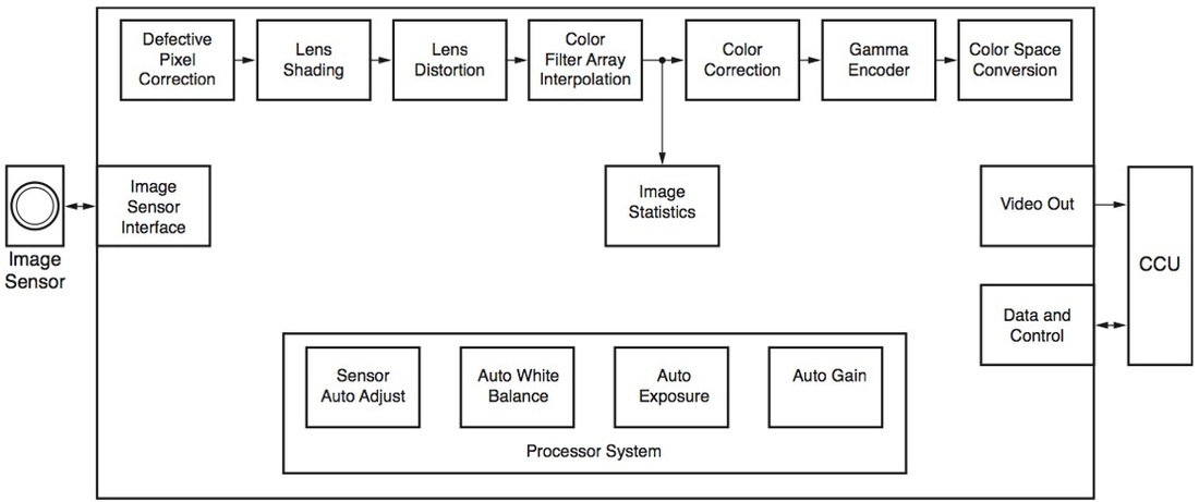
| endoscopy_block_diagram.pptx |
| block_diagram_explanation_endoscopy.docx |


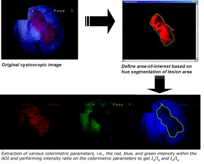
1) Color change detection
shade of red
shade of red

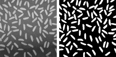
2) Image to black and white


| edge-detection.pdf |

Abstract:
A method for detecting possible presence of abnormality in the endoscopic images of lower esophagus is presented. The preprocessed endoscopic color images are segmented using color segmentation based on 3σ-intervals around mean RGB values. The zero-crossing method of edge detection is applied on the gray scale image corresponding to the segmented image. For the large contours, the Gaussian smoothing is performed for eliminating the noise in the curve. The curvature for each point of the curve is computed considering the support region of each point. The possible presence of abnormality is identified, when curvature of the contour segment between two zero crossing has the opposite curvature signs to those of such neighboring contour segments on the same edge contours. The experimental results show successful abnormality detection in the test images using this proposed method. 1 Introduction The technique of endoscopy has expanded the understanding of numerous gastrointestinal diseases since from its wide spread use in the late 1960s. The careful inspection of mucosa surface has greatly improved the ability to care the affected patients. As the video endoscope containing the intensity light source, suction equipment, guided camera, etc, passes under direct vision, through the esophagus and the stomach into a portion of duodenum, it transmits the video clipping of tissues for the display, the storage and the analysis. Endoscopy of lower gastrointestinal system provides real time image information about colorectal mucosa and is being used increasingly to identify abnormalities and disorders of the colon.
INTRODUCTION:
Endoscopy provides images better than that of the other tests, and in many cases endoscopy is superior to the other imaging techniques such as traditional x-rays. A physician may use an endoscopy as a tool for diagnosing the possible disorders in the digestive tract. Symptoms that may indicate the need for an endoscopy include swallowing difficulties, nausea, vomiting, reflux, bleeding, indigestion, abdominal pain, chest pain and a change in bowel habits. In the conventional approach for the diagnosis of endoscopic images the visual interpretation by the physician is employed. The process of computerized visualization, interpretation and analysis of endoscopic images will assist the physician for fast identification of the abnormality in the images [1]. In this direction research works are being carried out for classifying the abnormal endoscopic images based on their properties like color, texture, structural relationships between the image pixels, etc. The method proposed by P.Wang et.al.[2] classifies the endoscopic images based on texture and neural network, where as the analysis of curvature for the edges obtained from the endoscopic images is proposed by Krishnan et.al.[3]. Hiremath et.al.[4] proposed a method to detect the possible presence of abnormality using color segmentation of the images based on 3σ- for obtaining edges followed by curvature analysis. The watershed segmentation approach for classifying abnormal endoscopic images is proposed by Dhandra et.al.[6]. In this paper the active contours using the level set method with energy minimization approach, which is also known as active contours without edges proposed by chan et.al [7] is adopted for the segmentation of the endoscopic images followed by the curvature computation of the boundary of each obtained region. The zero crossings of the curvature plot for each edge are obtained for further analysis. In the following section we shall discuss the mathematical formulation for level set method and active contours without edges. In Section 3 the curvature analysis is discussed. In Section 4 the K nearest neighborhood classification is discussed.
Endoscopy provides images better than that of the other tests, and in many cases endoscopy is superior to the other imaging techniques such as traditional x-rays. A physician may use an endoscopy as a tool for diagnosing the possible disorders in the digestive tract. Symptoms that may indicate the need for an endoscopy include swallowing difficulties, nausea, vomiting, reflux, bleeding, indigestion, abdominal pain, chest pain and a change in bowel habits. In the conventional approach for the diagnosis of endoscopic images the visual interpretation by the physician is employed. The process of computerized visualization, interpretation and analysis of endoscopic images will assist the physician for fast identification of the abnormality in the images [1]. In this direction research works are being carried out for classifying the abnormal endoscopic images based on their properties like color, texture, structural relationships between the image pixels, etc. The method proposed by P.Wang et.al.[2] classifies the endoscopic images based on texture and neural network, where as the analysis of curvature for the edges obtained from the endoscopic images is proposed by Krishnan et.al.[3]. Hiremath et.al.[4] proposed a method to detect the possible presence of abnormality using color segmentation of the images based on 3σ- for obtaining edges followed by curvature analysis. The watershed segmentation approach for classifying abnormal endoscopic images is proposed by Dhandra et.al.[6]. In this paper the active contours using the level set method with energy minimization approach, which is also known as active contours without edges proposed by chan et.al [7] is adopted for the segmentation of the endoscopic images followed by the curvature computation of the boundary of each obtained region. The zero crossings of the curvature plot for each edge are obtained for further analysis. In the following section we shall discuss the mathematical formulation for level set method and active contours without edges. In Section 3 the curvature analysis is discussed. In Section 4 the K nearest neighborhood classification is discussed.

Literature:
A color WCE image is a snapshot of the digestive tract at a given time. However, in a computer-aided diagnosis system, the image content semantics needs to be translated in numerical ways for interpretation. There are several ways to represent the numerical form of an image known as image abstraction. Among WCE applications, there are three popular features for image abstraction: (1) color, (2) texture, and (3) shape features. Color images produced by WCE contain much useful color information and hence can be used as effective cue to suggest the topographic location of the current image. Figure 1 shows typical images taken from each organ. In this figure, the stomach looks pinkish, the small intestine is yellowish due to the slightly straw-color of the bile, and the colon is often yellowish or greenish due to the contamination of the liquid form of faeces. Another popular image abstraction feature in medical-imaging-related applications is the texture feature [2]. In WCE applications, a unique texture pattern called “villi” can be used to distinguish the small intestine from other organs. In addition, abnormality in WCE video can be discriminated by comparing the texture patterns between normal and abnormal mucosa regions, making texture pattern a popular feature for image abstraction. Shape feature is another commonly used abstraction approach for machine vision applications. Object shapes provide strong clues to object identity, and humans can recognize objects solely on their shapes. In the following subsections, we provide a high level survey of these features along with some popular implementations.
Color is a way the human visual system used to measure a range of the electromagnetic spectrum, which is approximately between 300 and 830 nm. The human visual system only recognizes certain combinations of the visible spectrum and associates these spectra into color. Today, a number of color models (e.g., RGB, HSI/HSV, CIE Lab, YUV, CMYK, and Luv) are available. Among all, the most popular color models in WCE applications are the RGB and HSI/HSV color models.The RGB color model is probably best known. Most image-capturing devices use the RGB model, and the color images are stored in forms of two-dimensional array of triplets made of red, blue, and green. There are a couple of characteristics that make the RGB model the basic color space: (1) existing methods to calibrate the image capturing devices and (2) multiple ways to transform the RGB model into a linear, perceptually uniform color model. On the other hand, the main disadvantage of RGB-based natural images is the high degree of correlation between their components, meaning that if the intensity changes, all three components will change accordingly.

Physiological background:
The innovation of wireless capsule endoscopy (CE) has revolutionized the investigation and management of patients with suspected small bowel disease [1]. Since its introduction, in the year 2000, a new chapter in the small bowel examination was opened, as this new technology allows the visualization of the entire gastrointestinal (GI) tract, reaching places where conventional endoscopy is unable to. In fact, conventional endoscopy presents some important limitations in the diagnosis of small bowel problems, since it is limited to the upper GI tract, at the duodenum, and to lower GI tract, at terminal ileum. Therefore, prior to the wireless capsule endoscopy era, the small intestine was the conventional endoscopy's last frontier, because it could not be internally visualized directly or in it's entirely by any method [2]. The small intestine accounts for 75% of the total length and 90% of the surface area of the gastrointestinal tract [3]. In adults it measures about 570 cm at post mortem, which is substantially longer than conventional video endoscopes (100-180 cm) [3]. Push enteroscopy (PE) is an effective diagnostic and therapeutic procedure, although it only allows exploration of the proximal small bowel [4]. Intraoperative enteroscopy is the most complete but also the most invasive means of examining the small bowel [5]. On the other hand, CE is a simple, non-invasive procedure that is well accepted by the patient and can be performed on an outpatient basis, allowing simultaneously the visualization of the entire GI tract. This technique is especially successful in finding bleeding regions, Crohn's disease and suspected tumors of the small bowel [2,6].
The first commercially-available wireless video capsule was the M2ATM (by Given Imaging Ltd., Yoqneam, Israel), a pill-like device (11 mm × 26 mm), which contains a miniaturized camera, a light source and a wireless circuit for the acquisition and transmission of signals [7]. The capsule is passively propelled trough the entire GI tract, through peristalsis, capturing images at a rate of two frames per second. Image features include a 140° field of view, 1:8 magnification allowing visualization of individual villi, 1-30 mm depth of view and a minimum size of detection of about 0.1 mm.
Current approaches rely in the fact that alterations in the texture of the small bowel mucosa can be used in automatic detection methods of abnormalities, which potentially indicate disease. These alterations are just what the physicians usually search for. For instance, Maroulis et al. and Karkanis et al. proposed two different methods based on the analysis of textural descriptors of wavelet coefficients in colonoscopy videos [14,15]. Indeed texture extraction algorithms can be used as feature sources of classifiers, in order to develop automatic classification schemes for CE video frames evaluation. Kodogiannis et al. proposed two different schemes to extract features from texture spectra in the chromatic and achromatic domains [16]. Although presented for a slightly different event detection, the works of Cunha et al. and Mackiewicz et al. suggest that a significant reduction of the viewing time can be achieved by automatic topographic segmentation the capsule endoscopic videos [17,18]. Szczypinski et al. have recently proposed a different and very interesting concept to aid clinicians in the interpretation of capsule endoscopic videos [19]. They propose the use of a model of deformable rings to compute motion-descriptive characteristics and to produce a two-dimensional representation of the GI tract's internal surface. From these maps, certain characteristics that indicate areas of bleeding, ulceration and obscuring froth can be easily recognized, allowing therefore the quick identification of such abnormal areas. Recently, a different approach has also been proposed by Iakovidis et al. to reduce the capsule endoscopic reading times, through the use of an unsupervised image mining technique [20]. Using a different rationale than the typical viewing time reduction, Karargyris and Bourbakis have recently proposed a method to enhance the video and therefore improve the viewing of the digestive tract, leading to a richer, more qualitative and efficient CE examination [21]. The detection of abnormalities, with special incidence in blood presence, in CE frames through computational approaches has been indeed a particularly active topic in the last few years [22-25]. For further notes on the available methodologies for CE image processing, the reader is advised to consult the recent review by Karargyris and Bourbakis [26]. In authors' previous work [27-30], different methods are proposed for classification of capsule endoscopic video frames based on statistical measures taken from texture descriptors of co-occurrence matrices, using the discrete wavelet transform to select the bands with the most significant texture information for classification purposes. Furthermore, the measurement of the non-Gaussianity of these statistical texture descriptors regarding marginal distributions was used in [29], in a classification scheme to identify abnormal frames. This paper proposes extending this approach to the joint distribution modeling, allowing to further explore the texture patterns in CE frames, having however the drawback of strongly increasing the dimensionality of the observation vector.

Working principle:
It is a technique to modify or interpret existing pictures, such as photographs. Two principal applications of image processing are:
1. Improving picture quality
2. Machine perception of visual information as used in robotics
Working of image processing: To apply image-processing methods, we first digitize a photograph or other picture into an image file. Then digital methods can be applied to rearrange picture parts, to enhance color separations, or to improve the quality of shading. An example of the application of image-processing methods is to enhance the quality of a picture. These techniques are used extensively in commercial art applications that involve the retouching and rearranging of sections of photographs and other artwork. Similar methods are used to analyze satellite photos of the earth and photos of galaxies.
There are several different types of endoscope. Each one is designed to investigate a specific part of the body. Endoscopes may be rigid or flexible, although most endoscopes in routine use are flexible. The two types differ in appearance, but function in similar ways. Both use light to magnify and view the internal structures of the body.
Flexible endoscopes are useful for looking at the digestive and respiratory tracts because they bend in places. They use fibre optics to shine light into the body. Fibre optics are thin strands of glass or plastic that transmit light by reflecting it. Water and air, as well as surgical instruments that may be necessary to take a tissue sample, can also be passed along the hollow centre of the endoscope.
Flexible endoscopes have a tiny camera attached to the end. The view recorded by the camera is displayed on a computer screen for the doctor, and sometimes the patient, to see.
Rigid endoscopes are usually much shorter than flexible endoscopes. They are often used to look at the surface of internal organs, and may be inserted through a small cut in the skin. Gas or fluid is sometimes used to move the surface tissues of organs in order to see them more clearly. Rigid endoscopes are commonly used to examine the joints.

Block diagram:
Future scope:
e recognised information is then relayed to users through attached headphones. "Human beings tend to process visual information faster and more accurately than text. A picture after all speaks a thousand words. Image processing will move the world, just how text search did last decade. Using object recognition, Imagenistics has come up with a unique visual search engine for complicated industrial products -- which are hard to describe in words -- to connect buyers and sellers in the industrial workplace. "Digital cameras in many cellphones today look at the same wave lengths of light as we ourselves see. But we will see many new kinds of other sensing modalities as well, which we are not so familiar with today," says Baraniuk. For instance, infra-red imaging, which is already very important in applications like inspecting packages, night-time security and in seeing through mist and heavy fog.
That pretty much is a sensor-data game. To realize its full potential, image processing needs billions of high-quality, cheaper sensors --which is already happening. But then, there's the consequence: how do you handle the humunguous data captured by these sensors? If lawmakers are hunting for a particular globe-trotting terrorist for instance, they have to go through the images and videos of hundreds of thousands of people at airports. These images and their processing require huge amounts of storage and energy, and are not even useful.
"The amount of data is growing faster than the amount of digital storage. Image processing's biggest challenge is coping with this data deluge, while continuing to build sensors with newer modalities and perfect algorithms to handle all of this," says Baraniuk. An answer has come in the form of a new field called compressed sensing,
Image processing has already begun to move our world. But for it to shift the axis, computers will have to see the way we do, and as Medioni and Barnauik concur, we still need decades of research to get close to that vision. Meanwhile, next time your faucet leaks, try clicking a picture and your favourite search engine could tell you where to order a new one from.
Advantages:
There are several advantages with digital cameras compared to other means of acquiring data. The key point for our purposes are the large spatial resolution of our CCD cameras. A resolution of pixels allows for a rather large span in the size of the features detected by the cameras. This is crucial for reliable fractal analysis of scaling relations. The size of the pixels of m is of the same order as the grain size in photographic films. The large number of other advantages of the CCD cameras therefore makes them superior to video cam-recorders or ordinary cameras. Digital cameras are extremely sensitive and have a high signal to noise ratio. In addition, digital cameras are stationary during an experiments which means that a given pixel images the same physical area when a series of images are captured. It is also possible to inspect the recorded image immediately after they have been captured, as opposed to ordinary photographic cameras where the films have to be developed.
The digital cameras have a linear intensity response, and no color filters complicate the analysis. This also makes these cameras suitable for applications such as when light intensities after absorption or fluorescence are used to map the height field. Ordinary photographic film has a logarithmic intensity response where the brightness depends on the amount of developer and time in developing baths, which makes them less suitable for intensity measurements.
Limitations:
1) It's very costly depending on the system used, the number of detectors purchased.
2) Time consuming
3) Lack of qualified professional
1) It's very costly depending on the system used, the number of detectors purchased.
2) Time consuming
3) Lack of qualified professional
Applications:
Endoscopic ultrasonography (EUS) employs the technology of endoscopy and internally placed high-frequency ultrasound waves to visualize the gastrointestinal wall and adjacent structures. Conventional EUS has 2 designs: the radial scanner and the sector scanner. In addition, high-frequency ultrasound probes that are passed through the biopsy channel of an endoscope are available. EUS has emerged as an important modality for the diagnosis and staging of benign and malignant lesions of the gut wall and surrounding structures of the mediastinum, abdomen, and pelvis. It is also used as a diagnostic tool for the evaluation of submucosal masses of the upper gastrointestinal tract and the rectosigmoid, for locating pancreatic endocrine tumors, and for the assessment of vascular disease. Interventional applications, such as EUS-guided fine-needle aspiration (EUS-FNA) for obtaining tissue/fluid samples, for pseudocyst drainage, and also for delivery of local therapy, will likely enhance the clinical utility and cost-effectiveness of this imaging modality. The widest application of EUS is, however, in the diagnosis and staging of esophageal, gastric, rectal, and pancreaticobiliary carcinoma. EUS has been shown to change the approach to clinical management in a significant proportion of patients to a less costly, risky, or invasive strategy. This article update reviews recent literature on the role of EUS in guiding FNA; in the diagnosis, staging, and management of patients with benign and malignant lesions of the gastrointestinal tract and adjacent structures; and in the assistance of interventions such as pseudocyst drainage and endoscopic mucosal resection.
Endoscopic ultrasonography (EUS) employs the technology of endoscopy and internally placed high-frequency ultrasound waves to visualize the gastrointestinal wall and adjacent structures. Conventional EUS has 2 designs: the radial scanner and the sector scanner. In addition, high-frequency ultrasound probes that are passed through the biopsy channel of an endoscope are available. EUS has emerged as an important modality for the diagnosis and staging of benign and malignant lesions of the gut wall and surrounding structures of the mediastinum, abdomen, and pelvis. It is also used as a diagnostic tool for the evaluation of submucosal masses of the upper gastrointestinal tract and the rectosigmoid, for locating pancreatic endocrine tumors, and for the assessment of vascular disease. Interventional applications, such as EUS-guided fine-needle aspiration (EUS-FNA) for obtaining tissue/fluid samples, for pseudocyst drainage, and also for delivery of local therapy, will likely enhance the clinical utility and cost-effectiveness of this imaging modality. The widest application of EUS is, however, in the diagnosis and staging of esophageal, gastric, rectal, and pancreaticobiliary carcinoma. EUS has been shown to change the approach to clinical management in a significant proportion of patients to a less costly, risky, or invasive strategy. This article update reviews recent literature on the role of EUS in guiding FNA; in the diagnosis, staging, and management of patients with benign and malignant lesions of the gastrointestinal tract and adjacent structures; and in the assistance of interventions such as pseudocyst drainage and endoscopic mucosal resection.
Conclusion:
Thus a computerized tumor detection system is used for WCE images. The proposed textural features use the advantages of mean and energy in discrete wavelet transform, working much better than traditional features for tumor detection in WCE images. By using SVM-RFE classifier, for 18 images tumor is detected. The classifier shows with 100% accuracy. So to obtain proper classification accuracy, more number of images are to be given in future. Also different classifiers viz. Naive Bayes classifier, Multi SVM will be incorporated and their performances are to be analyzed. As a result, the best classifier is preferred for tumor detection accuracy.
Thus a computerized tumor detection system is used for WCE images. The proposed textural features use the advantages of mean and energy in discrete wavelet transform, working much better than traditional features for tumor detection in WCE images. By using SVM-RFE classifier, for 18 images tumor is detected. The classifier shows with 100% accuracy. So to obtain proper classification accuracy, more number of images are to be given in future. Also different classifiers viz. Naive Bayes classifier, Multi SVM will be incorporated and their performances are to be analyzed. As a result, the best classifier is preferred for tumor detection accuracy.
Specifications:
- USB Connection - Camera connects to your computer via USB for efficient capturing of digital images, streamlining the transfer of images to your Electronic Health Records.
- Portable - Easily move the Camera and Light Source from room to room or office to office for improved time management and patient convenience.
- Simple to Use - Two button design allows for intuitive set up as well as for image or video capturing.
- Compatibility - The eN-CAM™ will work with almost any rigid or flexible Endoscope and plugs into most Laptops or Personal Computers (see Specifications).
- LED Light Source - This "size of your hand" compact LED Light Source ensures easy mobility, is brighter than halogen and almost completely quiet.
General Specifications: - Computer Specifications Requirements Windows XP Pro, Vista Business or Windows 7 Pro Operating System.
- Intel Core2 Processor, minimum 2GB RAM and 16GB storage, 4 USB 2.0 hi-speed ports and Intel or NEC USB chipsets. Nvidia or ATI graphical chipset with dedicated 128MB RAM with support for DirectX 9 as well as screen resolution of 1024 X 768 or higher.
- Camera Sensor Resolution 752 X 582 PAN and 768 X 494 NTSC, Definition is 470 lines and Sensitivity of 2 lux. Electronic Shutter is Automatic 1/50 to 1/100,000. Cable is 3 meters. Power Supply is 5 Volt DC. Camera head is ABS-PC waterproof.
- Light Source White (450°K) LED Light Source with 30 watts of power supplying an equivalent light output of a 100 watt Xenon Light Source. Life of LED is 50,000 hours with low power consumption and minimal noise.
Introduction to MAT-LAB:
MATLAB is a high-performance language for technical computing. It integrates computation, visualization, and programming in an easy-to-use environment where problems and solutions are expressed in familiar mathematical notation. Typical uses include:
The MATLAB system consists of five main parts: The MATLAB language. This is a high-level matrix/array language with control flow statements, functions, data structures, input/output, and object-oriented programming features. It allows both "programming in the small" to rapidly create quick and dirty throw-away programs, and "programming in the large" to create complete large and complex application programs. The MATLAB working environment. This is the set of tools and facilities that you work with as the MATLAB user or programmer. It includes facilities for managing the variables in your workspace and importing and exporting data. It also includes tools for developing, managing, debugging, and profiling M-files, MATLAB's applications.
Handle Graphics. This is the MATLAB graphics system. It includes high-level commands for two-dimensional and three-dimensional data visualization, image processing, animation, and presentation graphics. It also includes low-level commands that allow you to fully customize the appearance of graphics as well as to build complete Graphical User Interfaces on your MATLAB applications. The MATLAB mathematical function library. This is a vast collection of computational algorithms ranging from elementary functions like sum, sine, cosine, and complex arithmetic, to more sophisticated functions like matrix inverse, matrix eigenvalues, Bessel functions, and fast Fourier transforms. The MATLAB Application Program Interface (API). This is a library that allows you to write C and Fortran programs that interact with MATLAB. It include facilities for calling routines from MATLAB (dynamic linking), calling MATLAB as a computational engine, and for reading and writing MAT-files.
MATLAB is a high-performance language for technical computing. It integrates computation, visualization, and programming in an easy-to-use environment where problems and solutions are expressed in familiar mathematical notation. Typical uses include:
- Math and computation
- Algorithm development
- Modeling, simulation, and prototyping
- Data analysis, exploration, and visualization
- Scientific and engineering graphics
- Application development, including Graphical User Interface building
The MATLAB system consists of five main parts: The MATLAB language. This is a high-level matrix/array language with control flow statements, functions, data structures, input/output, and object-oriented programming features. It allows both "programming in the small" to rapidly create quick and dirty throw-away programs, and "programming in the large" to create complete large and complex application programs. The MATLAB working environment. This is the set of tools and facilities that you work with as the MATLAB user or programmer. It includes facilities for managing the variables in your workspace and importing and exporting data. It also includes tools for developing, managing, debugging, and profiling M-files, MATLAB's applications.
Handle Graphics. This is the MATLAB graphics system. It includes high-level commands for two-dimensional and three-dimensional data visualization, image processing, animation, and presentation graphics. It also includes low-level commands that allow you to fully customize the appearance of graphics as well as to build complete Graphical User Interfaces on your MATLAB applications. The MATLAB mathematical function library. This is a vast collection of computational algorithms ranging from elementary functions like sum, sine, cosine, and complex arithmetic, to more sophisticated functions like matrix inverse, matrix eigenvalues, Bessel functions, and fast Fourier transforms. The MATLAB Application Program Interface (API). This is a library that allows you to write C and Fortran programs that interact with MATLAB. It include facilities for calling routines from MATLAB (dynamic linking), calling MATLAB as a computational engine, and for reading and writing MAT-files.
Introduction to image processing:
Image processing is a method to convert an image into digital form and perform some operations on it, in order to get an enhanced image or to extract some useful information from it. It is a type of signal dispensation in which input is image, like video frame or photograph and output may be image or characteristics associated with that image. Usually Image Processing system includes treating images as two dimensional signals while applying already set signal processing methods to them.
It is among rapidly growing technologies today, with its applications in various aspects of a business. Image Processing forms core research area within engineering and computer science disciplines too. Image processing basically includes the following three steps. ·
Importing the image with optical scanner or by digital photography. ·
Analyzing and manipulating the image which includes data compression and image enhancement and spotting patterns that are not to human eyes like satellite photographs. ·
Output is the last stage in which result can be altered image or report that is based on image analysis.
The purpose of image processing is divided into 5 groups. They are:
1. Visualization - Observe the objects that are not visible.
2. Image sharpening and restoration - To create a better image.
3. Image retrieval - Seek for the image of interest.
4. Measurement of pattern – Measures various objects in an image.
5. Image Recognition – Distinguish the objects in an image.
Types
The two types of methods used for Image Processing are Analog and Digital Image Processing.
Analog or visual techniques of image processing can be used for the hard copies like printouts and photographs. Image analysts use various fundamentals of interpretation while using these visual techniques. The image processing is not just confined to area that has to be studied but on knowledge of analyst. Association is another important tool in image processing through visual techniques. So analysts apply a combination of personal knowledge and collateral data to image processing.
Digital Processing techniques help in manipulation of the digital images by using computers. As raw data from imaging sensors from satellite platform contains deficiencies. To get over such flaws and to get originality of information, it has to undergo various phases of processing. The three general phases that all types of data have to undergo while using digital technique are Pre- processing, enhancement and display, information extraction.
Enhancement methods in image processing:
Image enhancement is the process of adjusting digital images so that the results are more suitable for display or further image analysis. For example, you can remove noise, sharpen, or brighten an image, making it easier to identify key features.
Here are some useful examples and methods of image enhancement:
- Filtering with morphological operators
- Histogram equalization
- Noise removal using a Wiener filter
- Linear contrast adjustment
- Median filtering
- Unsharp mask filtering
- Contrast-limited adaptive histogram equalization (CLAHE)
- Decorrelation stretch
- The following images illustrate a few of these examples:

clear all
clc
close all
imtool close all
prefix = 'C:\Data\February14\24\img\'; %file name prefix
%A=input ('statring file number')
fnum = 1:15; %file numbers
ext = '.jpg'; %extension
fname = [prefix num2str(fnum(1)) ext];
%info = dicominfo(fname)
hWaitBar = waitbar(0,'Reading JPEG files');
for i=length(fnum):-1:1
fname = [prefix num2str(fnum(i)) ext];
D(:,:,:,i) = uint8(imread(fname));
waitbar((length(fnum)-i)/length(fnum))
end
delete(hWaitBar)
whos D
%% Visualization
%----------------------------------------------------------------------
%explore image data using Image Viewer GUI tool
for i1=1:1:15
%i1 = 1; %middle slice
im = squeeze(D(:,:,i1));
max_level = double(max(D(:)));
imtool(im,[0 max_level])
%custom display - image data
fig1 = figure;
max_level = double(max(D(:)));
imshow(im,[0 max_level])
title('Coronal Slice #1')
set(fig1,'position',[601 58 392 314])
%imtool close all
%add intensity legend
colorbar
%change colormap
colormap jet
I= D(:,:,:,i1);
figure(),
imshow(I);
[m,n,z]=size(I);
%% color extraction
Ir=uint8(zeros(m,n,z));
Ig=uint8(zeros(m,n,z));
Ib=uint8(zeros(m,n,z));
Ir(:,:,1)=I(:,:,1);
Ig(:,:,2)=I(:,:,2);
Ib(:,:,3)=I(:,:,3);
figure(),
imshow(Ir);
figure(),
imshow(Ig);
figure(),
imshow(Ib);
redimage=I(:,:,1);
greenimage=I(:,:,2);
blueimage=I(:,:,3);
figure(),
imshow(redimage);
figure(),
imshow(greenimage);
figure(),
imshow(blueimage);
figure()
imhist(redimage)
figure()
imhist(greenimage)
figure()
imhist(blueimage)
%% Eulars algorithm
a = histeq(redimage);
b=255;
trans_thresh = mrdivide(0:1:b,b); % Here is to set an array for calculating different euler number
%mrdevide is A/B is the matrix division of B into A, which is roughly the same as A*INV(B) , except it is computed in a different way.
% 0/255 , 1/255, 2/255 ...and so on
for j=1:(b+1)
value_trans1 = trans_thresh(1,j);
result4_trans1(j,1) = bweuler(im2bw(a,value_trans1),4);
end
max_result4_trans1 = max(result4_trans1); % Calculating max of euler number
min_result4_trans1 = min(result4_trans1); % Calculating min of euler number
m = 0;
n = 0;
max_sum_result4_trans1 = 0;
min_sum_result4_trans1 = 0;
for j = 1:(b+1)
if result4_trans1(j,1) == max_result4_trans1
m = m+1;
max_sum_result4_trans1 = max_sum_result4_trans1 + j;
elseif result4_trans1(j,1) == min_result4_trans1
n = n+1;
min_sum_result4_trans1 = min_sum_result4_trans1 + j;
else
%Should Do Nothing Here
end
end
% Getting the mean of the threshold
threshold_I1 = ((max_sum_result4_trans1)+(min_sum_result4_trans1))/(m+n);
cred = im2bw(a,floor(1*threshold_I1)/(b+1));
figure()
imshow(cred);
a = histeq(greenimage);
b=255;
trans_thresh = mrdivide(0:1:b,b); % Here is to set an array for
% calculating different euler number
for j=1:(b+1)
value_trans1 = trans_thresh(1,j);
result4_trans1(j,1) = bweuler(im2bw(a,value_trans1),4);% 4 connected piexls
end
max_result4_trans1 = max(result4_trans1); % Calculating max of euler number
min_result4_trans1 = min(result4_trans1); % Calculating min of euler number
m = 0;
n = 0;
max_sum_result4_trans1 = 0;
min_sum_result4_trans1 = 0;
for j = 1:(b+1)
if result4_trans1(j,1) == max_result4_trans1
m = m+1;
max_sum_result4_trans1 = max_sum_result4_trans1 + j;
elseif result4_trans1(j,1) == min_result4_trans1
n = n+1;
min_sum_result4_trans1 = min_sum_result4_trans1 + j;
else
%Should Do Nothing Here
end
end
% Getting the mean of the threshold
threshold_I1 = ((max_sum_result4_trans1)+(min_sum_result4_trans1))/(m+n);
cgreen = im2bw(a,floor(1*threshold_I1)/(b+1));
figure()
imshow(cgreen);
a = histeq(blueimage);
b=255;
trans_thresh = mrdivide(0:1:b,b); % Here is to set an array for
% calculating different euler number
for j=1:(b+1)
value_trans1 = trans_thresh(1,j);
result4_trans1(j,1) = bweuler(im2bw(a,value_trans1),4);% 4 connected piexls
end
max_result4_trans1 = max(result4_trans1); % Calculating max of euler number
min_result4_trans1 = min(result4_trans1); % Calculating min of euler number
m = 0;
n = 0;
max_sum_result4_trans1 = 0;
min_sum_result4_trans1 = 0;
for j = 1:(b+1)
if result4_trans1(j,1) == max_result4_trans1
m = m+1;
max_sum_result4_trans1 = max_sum_result4_trans1 + j;
elseif result4_trans1(j,1) == min_result4_trans1
n = n+1;
min_sum_result4_trans1 = min_sum_result4_trans1 + j;
else
%Should Do Nothing Here
end
end
% Getting the mean of the threshold
threshold_I1 = ((max_sum_result4_trans1)+(min_sum_result4_trans1))/(m+n);
cblue = im2bw(a,floor(1*threshold_I1)/(b+1));
figure()
imshow(cblue);
end
|
| ||
Blackbook:-
