Introduction
Forensic art is any art used in law enforcement or legal proceedings. Within this field are such skills as composite drawing, crime scene sketching, image modification and image identification, courtroom drawings, demonstrative evidence, and postmortem and facial approximation aids. Not every forensic artist uses all of these skills.[1]
The term forensic comes from the Roman forum where law and politics were debated.[2] From this beginning, the word forensic now means anything pertaining to law or law enforcement or debate.[3]
The skill of facial approximation is closely associated and related to forensic anthropology in that an artist specializes in the reconstruction of the remains of a human body. Generally this discipline focuses on the human face for identification purposes. The forensic artist can create a facial approximation in a number of ways to include 2D (drawing), 3D (sculpture) and by methods using new computerized technology. Forensic artists generally can add greater character and make their subjects come back to "life".
Most forensic artists do the job as a collateral duty to their "regular" job in law enforcement, such as police officer, crime scene tech, etc. They do the work on salary, and normally are not paid extra for it. There are extremely few full-time forensic artist jobs to be had. Most full-time artists work in large cities, or in state or federal agencies. "Freelancing" in forensic art is extremely difficult to build as a career, as ties to law enforcement are a necessary part of the job, and agencies have limited budgets to pay contractors.

To better understand what forensic art is, it helps to know what forensic artists do, which is, Composite Imagery, Age Progressions and Image Modifications, Facial Approximations from the Skull, Post-Mortem Imagery, and Demonstrative Evidence (such as trial charts used in the courtroom)
1.1 Composites
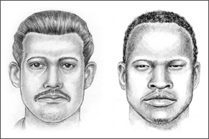
COMPOSITES are the one type of forensic art that you are probably the most are familiar with. These are the drawings or computer images that you see in the newspaper with headlines like, ”composite sketch released in search of robbery suspect” or “suspect sketch released in area stabbing incident.”
Traditionally, a “composite sketch” meant that the image was hand-drawn by an artist with pencil and paper, and a “composite image” was assembled with a computer application. With the advances in software technology, those distinctions have become blurred. Now, artists can draw directly on a computer screen with a digital pencil, and computer operators can assemble sketch-like images without ever having taken an art course. Sometimes it’s difficult to determine exactly how a composite was created just by looking at it anymore, and in the end it really doesn’t matter. Whether it’s called a composite sketch, drawing, or image, the purpose is the same: to provide police with leads to the identity of the person depicted.
Most artists still use pencil and paper, which requires no small amount of talent, and training in the cognitive interview process. Generally the computer-based systems were created to serve agencies that did not have a forensic artist and therefore “no artistic skill is needed to create the image”…. which can have mixed results. But to be fair, not all of us artists hit the drawing out of the park every time either, so there you go.
Composite are not portraits, and given the circumstances under which they’re produced, there’s no possible way they could be. And they certainly aren’t representative of how a forensic artist can draw when they’re off the clock.
We aren’t drawing what’s in front of us. That’s a piece of cake. Instead, what we’re doing is drawing what another person saw, when they were likely in the midst of one of the most terrifying moments of their life: being the victim or witness to a crime. Our job is to pull the memory of the face of their attacker out of their mind, and put it down on paper.
Every line we draw, every stroke we make on the paper is subject to being changed by the witness, at any point during the drawing session to make it look like the image in their head. For a forensic artist, an eraser is used every bit as much as the pencil. And that means the drawing isn’t going to look exactly the way we want it to.
This brings out another point about being a forensic artist. There’s no room for ego in this line of work. We know our skills, and we know we can draw pretty pictures of pretty people. But when the witness describes a person with buggy eyes, giraffe-like neck, and their hair in pigtails, then that’s exactly what we’re going to draw. It’s not quite fair if that sketch ends up on “Tosh.0”, but it’s what we have to accept as part of the job.
A composite drawing is more of a technical illustration as opposed to fine art; it’s a visual statement of what another person saw, or more accurately, what they perceived seeing. Because we are working from someone’s memory, it’s going to be nearly impossible to get a perfect likeness, even if that person were describing their own mother. Under the best of circumstances, it’s more likely that we are going to get a general resemblance to the suspect, something that looks close to what that person looked like.
And just like horseshoes and hand grenades, “close” counts in a composite drawing. A composite has done its job if it figuratively taps someone on the shoulder and says “you might need to pay attention to this.” It’s enough if someone watching the news about last night’s shooting thinks, “that looks an awful lot like Carl and he acted pretty jumpy when I asked him why it took so long to come back from the dry-cleaners.”
And of course, the drawing has really done its job if that person picks up the phone and calls the number on the TV.
Age Progression

AGE PROGRESSIONS of adults are pretty much what they sound like: “He’s been gone for 15 years, so take this photo and make him look like he’s 50 years old and balding.” These are done in cases of endangered missing adults as well as fugitives, all in the hopes of generating renewed public interest and fresh leads for investigators. I hate to burst anyone’s bubble, but forensic artists don’t have any special gifts or psychic ability to predict what someone will look like in the future. What we do have is in-depth knowledge of facial anatomy, we’ve studied aging patterns of the face, and we have the artistic ability to illustrate those changes.
Barring any new specific information about a person’s appearance, it comes down to educated guesswork. It’s sort of like the cliché in any time travel movie: what we produce is a vision of one possible future. Any number of things along the way can change the outcome.
So why bother with an age progression in the first place? Because the investigator has a case that’s gone cold, and an age-progressed image can be just the thing that heats it up again. It can provide a fresh look to a case that many people have long forgotten, and can be enough to get the media interested as well. Which is exactly what the investigator is after.
To create an age-progressed image, whether by retouching the photo or doing a drawing, an artist follows the same basic protocol. First, you try to get as much information on the person as possible, such as their lifestyle, genetics, occupation, etc. The more information, the better.
This is because you would age someone differently if they were an outdoorsy and athletic person, versus someone that had an office job and was prone to overweight. Every forensic artist should have a strong knowledge of anatomy, and keen observational skills. For instance, there can be extremely subtle differences in how a person looks change from their 30’s into their 40’s. An artist needs to make the image look real and believeable, and not just an image where it looks like wrinkles have been painted on.
Whether hand drawn or produced with the use of Photoshop, age progressions are just one of several possible “looks’ that a person may have when they age. Forensic artists are not psychic, and there is no guarantee that what is produced will look 100%, or even 75% of what the person may look like when apprehended. But, with a motivated law enforcement team putting the image out there to the public, this can often generate enough interest that people will take a second look, and call in a lead.
Every forensic artist has a story to tell where the detective hits a dead end on their investigation, and is now pinning their hopes that an artist’s age progression will get their case on the evening news, or the granddaddy of them all, America’s Most Wanted. Twenty years of searching have often come to an abrupt, satisfying end for the investigator just minutes after their fugitive’s image flashes on screen.

AGE PROGRESSIONS of children come with their own special set of circumstances. Needless to say, the aging process for adults is vastly different than that of children, so the method for producing an age-progressed image of a child is different as well. Instead of lifestyle changes, artists must depict the proportional changes of a child’s growth. This requires specialized knowledge, and ideally, specific input from the missing child’s parents and siblings. Many cases of child abductions are a result of custody disputes so this input isn’t always available, but continually updated images of the missing child are a way to help keep the search alive, and in the public’s memory.
Literature Review

Methodology
Syntax
A = imread(filename, fmt)
[X, map] = imread(...)
[...] = imread(filename)
[...] = imread(URL,...)
[...] = imread(...,Param1,Val1,Param2,Val2...)
Description
A = imread(filename, fmt) reads a grayscale or color image from the file specified by the string filename. If the file is not in the current folder, or in a folder on the MATLAB® path, specify the full pathname.
The text string fmt specifies the format of the file by its standard file extension. For example, specify 'gif' for Graphics Interchange Format files. To see a list of supported formats, with their file extensions, use the imformats function. If imread cannot find a file named filename, it looks for a file named filename.fmt.
The return value A is an array containing the image data. If the file contains a grayscale image, A is an M-by-N array. If the file contains a truecolor image, A is an M-by-N-by-3 array. For TIFF files containing color images that use the CMYK color space, A is an M-by-N-by-4 array. See TIFF in the Format-Specific Information section for more information.
The class of A depends on the bits-per-sample of the image data, rounded to the next byte boundary. For example, imread returns 24-bit color data as an array of uint8 data because the sample size for each color component is 8 bits. See Tips for a discussion of bitdepths, and see Format-Specific Information for more detail about supported bit depths and sample sizes for a particular format.
[X, map] = imread(...) reads the indexed image in filename into X and its associated colormap into map. Colormap values in the image file are automatically rescaled into the range [0,1].
[...] = imread(filename) attempts to infer the format of the file from its content.
[...] = imread(URL,...) reads the image from an Internet URL. The URL must include the protocol type (e.g., http://).
[...] = imread(...,Param1,Val1,Param2,Val2...) specifies parameters that control various characteristics of the operations for specific formats. For more information, see Format-Specific Information.
Syntax
imshow(I)example
imshow(I,[low high])
imshow(I,[])
imshow(X,map)example
imshow(filename)example
imshow(___,Name,Value)
himage = imshow(___)
Description
example
imshow(I) displays image I in a Handle Graphics® figure, where I is a grayscale, RGB (truecolor), or binary image. For binary images, imshow displays pixels with the value 0 (zero) as black and 1 as white. imshow optimizes figure, axes, and image object properties for image display.
imshow(I,[low high]) displays the grayscale image I, where [low high] is a two-element vector that specifies the display range for I. The value low (and any value less than low) displays as black and the value high (and any value greater than high) displays as white. imshow displays values in between as intermediate shades of gray.
imshow(I,[]) displays the grayscale image I, where [] is an empty matrix that specifies that you want imshow to scale the image based on the range of pixel values in I, using [min(I(:)) max(I(:))] as the display range.
example
imshow(X,map) displays the indexed image X with the colormap map. A colormap matrix can have any number of rows, but it must have exactly 3 columns. Each row is interpreted as a color, with the first element specifying the intensity of red light, the second green, and the third blue. Color intensity can be specified on the interval 0.0 to 1.0.
example
imshow(filename) displays the image stored in the graphics file specified by filename.
imshow(___,Name,Value) displays an image, using name-value pairs to control aspects of the operation.
himage = imshow(___) returns the handle to the image object created by imshow.


SyntaxBW = im2bw(I, level)
BW = im2bw(X, map, level)
BW = im2bw(RGB, level)
DescriptionBW = im2bw(I, level) converts the grayscale image I to a binary image. The output image BW replaces all pixels in the input image with luminance greater than level with the value 1 (white) and replaces all other pixels with the value 0 (black). Specify level in the range [0,1]. This range is relative to the signal levels possible for the image's class. Therefore, a level value of 0.5 is midway between black and white, regardless of class. To compute the levelargument, you can use the function graythresh. If you do not specify level, im2bw uses the value 0.5.
BW = im2bw(X, map, level) converts the indexed image X with colormap map to a binary image.
BW = im2bw(RGB, level) converts the truecolor image RGB to a binary image.
If the input image is not a grayscale image, im2bw converts the input image to grayscale, and then converts this grayscale image to binary by thresholding.
Syntaxlevel = graythresh(I)
[level EM] = graythresh(I)
Descriptionlevel = graythresh(I) computes a global threshold (level) that can be used to convert an intensity image to a binary image with im2bw. level is a normalized intensity value that lies in the range [0, 1].
The graythresh function uses Otsu's method, which chooses the threshold to minimize the intraclass variance of the black and white pixels.
Multidimensional arrays are converted automatically to 2-D arrays using reshape. The graythresh function ignores any nonzero imaginary part of I.
[level EM] = graythresh(I) returns the effectiveness metric, EM, as the second output argument. The effectiveness metric is a value in the range [0 1] that indicates the effectiveness of the thresholding of the input image. The lower bound is attainable only by images having a single gray level, and the upper bound is attainable only by two-valued images.
SyntaxBW = edge(I)
gpuarrayBW = edge(gpuarrayI)
BW = edge(I,'sobel')
BW = edge(I,'sobel',thresh)
BW = edge(I,'sobel',thresh,direction)
BW = edge(I,'sobel',...,options)
[BW,thresh] = edge(I,'sobel',...)
BW = edge(I,'prewitt')
BW = edge(I,'prewitt',thresh)
BW = edge(I,'prewitt',thresh,direction)
[BW,thresh] = edge(I,'prewitt',...)
BW = edge(I,'roberts')
BW = edge(I,'roberts',thresh)
BW = edge(I,'roberts',...,options)
[BW,thresh] = edge(I,'roberts',...)
BW = edge(I,'log')
BW = edge(I,'log',thresh)
BW = edge(I,'log',thresh,sigma)
[BW,thresh] = edge(I,'log',...)
BW = edge(I,'zerocross',thresh,h)
[BW,thresh] = edge(I,'zerocross',...)
BW = edge(I,'canny')
BW = edge(I,'canny',thresh)
BW = edge(I,'canny',thresh,sigma)
[BW,thresh] = edge(I,'canny',...)
DescriptionBW = edge(I) takes an intensity or a binary image I as its input, and returns a binary image BW of the same size as I, with 1's where the function finds edges in I and 0's elsewhere.
gpuarrayBW = edge(gpuarrayI) performs the edge detection on a GPU. The input image and the output image are gpuArrays. This syntax requires the Parallel Computing Toolbox™.
By default, edge uses the Sobel method to detect edges but the following provides a complete list of all the edge-finding methods supported by this function:
Sobel MethodBW = edge(I,'sobel') specifies the Sobel method.
BW = edge(I,'sobel',thresh) specifies the sensitivity threshold for the Sobel method. edge ignores all edges that are not stronger than thresh. If you do not specify thresh, or if thresh is empty ([]), edge chooses the value automatically.
BW = edge(I,'sobel',thresh,direction) specifies the direction of detection for the Sobel method. direction is a string specifying whether to look for 'horizontal' or 'vertical' edges or 'both' (the default).
BW = edge(I,'sobel',...,options) provides an optional string input. String 'nothinning' speeds up the operation of the algorithm by skipping the additional edge thinning stage. By default, or when 'thinning' string is specified, the algorithm applies edge thinning.
[BW,thresh] = edge(I,'sobel',...) returns the threshold value.
Prewitt MethodBW = edge(I,'prewitt') specifies the Prewitt method.
BW = edge(I,'prewitt',thresh) specifies the sensitivity threshold for the Prewitt method. edge ignores all edges that are not stronger than thresh. If you do not specify thresh, or if thresh is empty ([]), edge chooses the value automatically.
BW = edge(I,'prewitt',thresh,direction) specifies the direction of detection for the Prewitt method. directionis a string specifying whether to look for 'horizontal' or 'vertical' edges or 'both' (default).
[BW,thresh] = edge(I,'prewitt',...) returns the threshold value.
Roberts MethodBW = edge(I,'roberts') specifies the Roberts method.
BW = edge(I,'roberts',thresh) specifies the sensitivity threshold for the Roberts method. edge ignores all edges that are not stronger than thresh. If you do not specify thresh, or if thresh is empty ([]), edge chooses the value automatically.
BW = edge(I,'roberts',...,options) where options can be the text string 'thinning' or 'nothinning'. When you specify 'thinning', or don't specify a value, the algorithm applies edge thinning. Specifying the 'nothinning'option can speed up the operation of the algorithm by skipping the additional edge thinning stage.
[BW,thresh] = edge(I,'roberts',...) returns the threshold value.
Laplacian of Gaussian MethodBW = edge(I,'log') specifies the Laplacian of Gaussian method.
BW = edge(I,'log',thresh) specifies the sensitivity threshold for the Laplacian of Gaussian method. edge ignores all edges that are not stronger than thresh. If you do not specify thresh, or if thresh is empty ([]), edge chooses the value automatically. If you specify a threshold of 0, the output image has closed contours, because it includes all the zero crossings in the input image.
BW = edge(I,'log',thresh,sigma) specifies the Laplacian of Gaussian method, using sigma as the standard deviation of the LoG filter. The default sigma is 2; the size of the filter is n-by-n, where n = ceil(sigma*3)*2+1.
[BW,thresh] = edge(I,'log',...) returns the threshold value.
Zero-Cross MethodBW = edge(I,'zerocross',thresh,h) specifies the zero-cross method, using the filter h. thresh is the sensitivity threshold; if the argument is empty ([]), edge chooses the sensitivity threshold automatically. If you specify a threshold of 0, the output image has closed contours, because it includes all the zero crossings in the input image.
[BW,thresh] = edge(I,'zerocross',...) returns the threshold value.
Canny Method
BW = edge(I,'canny',thresh) specifies sensitivity thresholds for the Canny method. thresh is a two-element vector in which the first element is the low threshold, and the second element is the high threshold. If you specify a scalar forthresh, this scalar value is used for the high threshold and 0.4*thresh is used for the low threshold. If you do not specify thresh, or if thresh is empty ([]), edge chooses low and high values automatically. The value for thresh is relative to the highest value of the gradient magnitude of the image.
BW = edge(I,'canny',thresh,sigma) specifies the Canny method, using sigma as the standard deviation of the Gaussian filter. The default sigma is sqrt(2); the size of the filter is chosen automatically, based on sigma.
[BW,thresh] = edge(I,'canny',...) returns the threshold values as a two-element vector.
Code Generationedge supports the generation of efficient, production-quality C/C++ code from MATLAB. When generating code, themethod, direction, and sigma arguments must be a compile-time constants. In addition, nonprogrammatic syntaxes are not supported. For example, the syntax edge(im), where edge does not return a value but displays an image instead, is not supported. Generated code for this function uses a precompiled platform-specific shared library. To see a complete list of toolbox functions that support code generation.
gpuarrayBW = edge(gpuarrayI)
BW = edge(I,'sobel')
BW = edge(I,'sobel',thresh)
BW = edge(I,'sobel',thresh,direction)
BW = edge(I,'sobel',...,options)
[BW,thresh] = edge(I,'sobel',...)
BW = edge(I,'prewitt')
BW = edge(I,'prewitt',thresh)
BW = edge(I,'prewitt',thresh,direction)
[BW,thresh] = edge(I,'prewitt',...)
BW = edge(I,'roberts')
BW = edge(I,'roberts',thresh)
BW = edge(I,'roberts',...,options)
[BW,thresh] = edge(I,'roberts',...)
BW = edge(I,'log')
BW = edge(I,'log',thresh)
BW = edge(I,'log',thresh,sigma)
[BW,thresh] = edge(I,'log',...)
BW = edge(I,'zerocross',thresh,h)
[BW,thresh] = edge(I,'zerocross',...)
BW = edge(I,'canny')
BW = edge(I,'canny',thresh)
BW = edge(I,'canny',thresh,sigma)
[BW,thresh] = edge(I,'canny',...)
DescriptionBW = edge(I) takes an intensity or a binary image I as its input, and returns a binary image BW of the same size as I, with 1's where the function finds edges in I and 0's elsewhere.
gpuarrayBW = edge(gpuarrayI) performs the edge detection on a GPU. The input image and the output image are gpuArrays. This syntax requires the Parallel Computing Toolbox™.
By default, edge uses the Sobel method to detect edges but the following provides a complete list of all the edge-finding methods supported by this function:
- The Sobel method finds edges using the Sobel approximation to the derivative. It returns edges at those points where the gradient of I is maximum.
- The Prewitt method finds edges using the Prewitt approximation to the derivative. It returns edges at those points where the gradient of I is maximum.
- The Roberts method finds edges using the Roberts approximation to the derivative. It returns edges at those points where the gradient of I is maximum.
- The Laplacian of Gaussian method finds edges by looking for zero crossings after filtering I with a Laplacian of Gaussian filter.
- The zero-cross method finds edges by looking for zero crossings after filtering I with a filter you specify.
- The Canny method finds edges by looking for local maxima of the gradient of I. The gradient is calculated using the derivative of a Gaussian filter. The method uses two thresholds, to detect strong and weak edges, and includes the weak edges in the output only if they are connected to strong edges. This method is therefore less likely than the others to be fooled by noise, and more likely to detect true weak edges.
Sobel MethodBW = edge(I,'sobel') specifies the Sobel method.
BW = edge(I,'sobel',thresh) specifies the sensitivity threshold for the Sobel method. edge ignores all edges that are not stronger than thresh. If you do not specify thresh, or if thresh is empty ([]), edge chooses the value automatically.
BW = edge(I,'sobel',thresh,direction) specifies the direction of detection for the Sobel method. direction is a string specifying whether to look for 'horizontal' or 'vertical' edges or 'both' (the default).
BW = edge(I,'sobel',...,options) provides an optional string input. String 'nothinning' speeds up the operation of the algorithm by skipping the additional edge thinning stage. By default, or when 'thinning' string is specified, the algorithm applies edge thinning.
[BW,thresh] = edge(I,'sobel',...) returns the threshold value.
Prewitt MethodBW = edge(I,'prewitt') specifies the Prewitt method.
BW = edge(I,'prewitt',thresh) specifies the sensitivity threshold for the Prewitt method. edge ignores all edges that are not stronger than thresh. If you do not specify thresh, or if thresh is empty ([]), edge chooses the value automatically.
BW = edge(I,'prewitt',thresh,direction) specifies the direction of detection for the Prewitt method. directionis a string specifying whether to look for 'horizontal' or 'vertical' edges or 'both' (default).
[BW,thresh] = edge(I,'prewitt',...) returns the threshold value.
Roberts MethodBW = edge(I,'roberts') specifies the Roberts method.
BW = edge(I,'roberts',thresh) specifies the sensitivity threshold for the Roberts method. edge ignores all edges that are not stronger than thresh. If you do not specify thresh, or if thresh is empty ([]), edge chooses the value automatically.
BW = edge(I,'roberts',...,options) where options can be the text string 'thinning' or 'nothinning'. When you specify 'thinning', or don't specify a value, the algorithm applies edge thinning. Specifying the 'nothinning'option can speed up the operation of the algorithm by skipping the additional edge thinning stage.
[BW,thresh] = edge(I,'roberts',...) returns the threshold value.
Laplacian of Gaussian MethodBW = edge(I,'log') specifies the Laplacian of Gaussian method.
BW = edge(I,'log',thresh) specifies the sensitivity threshold for the Laplacian of Gaussian method. edge ignores all edges that are not stronger than thresh. If you do not specify thresh, or if thresh is empty ([]), edge chooses the value automatically. If you specify a threshold of 0, the output image has closed contours, because it includes all the zero crossings in the input image.
BW = edge(I,'log',thresh,sigma) specifies the Laplacian of Gaussian method, using sigma as the standard deviation of the LoG filter. The default sigma is 2; the size of the filter is n-by-n, where n = ceil(sigma*3)*2+1.
[BW,thresh] = edge(I,'log',...) returns the threshold value.
Zero-Cross MethodBW = edge(I,'zerocross',thresh,h) specifies the zero-cross method, using the filter h. thresh is the sensitivity threshold; if the argument is empty ([]), edge chooses the sensitivity threshold automatically. If you specify a threshold of 0, the output image has closed contours, because it includes all the zero crossings in the input image.
[BW,thresh] = edge(I,'zerocross',...) returns the threshold value.
Canny Method
- Note: Not supported on a GPU.
BW = edge(I,'canny',thresh) specifies sensitivity thresholds for the Canny method. thresh is a two-element vector in which the first element is the low threshold, and the second element is the high threshold. If you specify a scalar forthresh, this scalar value is used for the high threshold and 0.4*thresh is used for the low threshold. If you do not specify thresh, or if thresh is empty ([]), edge chooses low and high values automatically. The value for thresh is relative to the highest value of the gradient magnitude of the image.
BW = edge(I,'canny',thresh,sigma) specifies the Canny method, using sigma as the standard deviation of the Gaussian filter. The default sigma is sqrt(2); the size of the filter is chosen automatically, based on sigma.
[BW,thresh] = edge(I,'canny',...) returns the threshold values as a two-element vector.
Code Generationedge supports the generation of efficient, production-quality C/C++ code from MATLAB. When generating code, themethod, direction, and sigma arguments must be a compile-time constants. In addition, nonprogrammatic syntaxes are not supported. For example, the syntax edge(im), where edge does not return a value but displays an image instead, is not supported. Generated code for this function uses a precompiled platform-specific shared library. To see a complete list of toolbox functions that support code generation.
Syntaxlevel = graythresh(I)
[level EM] = graythresh(I)
Descriptionlevel = graythresh(I) computes a global threshold (level) that can be used to convert an intensity image to a binary image with im2bw. level is a normalized intensity value that lies in the range [0, 1].
The graythresh function uses Otsu's method, which chooses the threshold to minimize the intraclass variance of the black and white pixels.
Multidimensional arrays are converted automatically to 2-D arrays using reshape. The graythresh function ignores any nonzero imaginary part of I.
[level EM] = graythresh(I) returns the effectiveness metric, EM, as the second output argument. The effectiveness metric is a value in the range [0 1] that indicates the effectiveness of the thresholding of the input image. The lower bound is attainable only by images having a single gray level, and the upper bound is attainable only by two-valued images.
[level EM] = graythresh(I)
Descriptionlevel = graythresh(I) computes a global threshold (level) that can be used to convert an intensity image to a binary image with im2bw. level is a normalized intensity value that lies in the range [0, 1].
The graythresh function uses Otsu's method, which chooses the threshold to minimize the intraclass variance of the black and white pixels.
Multidimensional arrays are converted automatically to 2-D arrays using reshape. The graythresh function ignores any nonzero imaginary part of I.
[level EM] = graythresh(I) returns the effectiveness metric, EM, as the second output argument. The effectiveness metric is a value in the range [0 1] that indicates the effectiveness of the thresholding of the input image. The lower bound is attainable only by images having a single gray level, and the upper bound is attainable only by two-valued images.
clc
close all
clear all
I= imread('C:\Data\October\15\1.jpg');
figure(),imshow(I);
I1=rgb2gray(I);
figure(),imshow(I1);
level=graythresh(I1);
I1=im2bw(I1,level);
figure(),imshow(I1);
[m1,n1]=size(I1);
I= imread('C:\Data\October\15\1\2.jpg');
figure(),imshow(I);
I2=rgb2gray(I);
figure(),imshow(I2);
I3=edge(I2,'Canny');
figure(),imshow(I3);
I4=~I3;
figure(),imshow(I4);
[m2 n2]=size(I4);
if(m2>m1)
I4=imresize(I4,m1/m2);
else
I4=imresize(I4,m1/m2);
end
threshdiff=abs(I4-I1);
threshdiff=sum(sum(threshdiff));
I= imread('C:\Data\October\15\1\4.jpg');
figure(),imshow(I);
I2=rgb2gray(I);
figure(),imshow(I2);
I3=edge(I2,'Canny');
figure(),imshow(I3);
I4=~I3;
figure(),imshow(I4);
[m2 n2]=size(I4);
if(m2<n2)
I4=I4';
else
end
if(m2>m1)
I4=imresize(I4,m1/m2);
else
end
threshdiff2=abs(I4-I1);
threshdiff2=sum(sum(threshdiff2));
